Simple 2D Pose Graph Example
Python and C++ code of this example can be found at pose_graph_example.py and pose_graph_example.cpp respectively.
Here we give a simple example of using factor graph to solve a small 2D pose graph problem. The problem is shown in figure below, where a vehicle moves forward on a 2D plane, makes a 270 degrees right turn, and has a relative pose loop closure measurement which is shown in red.
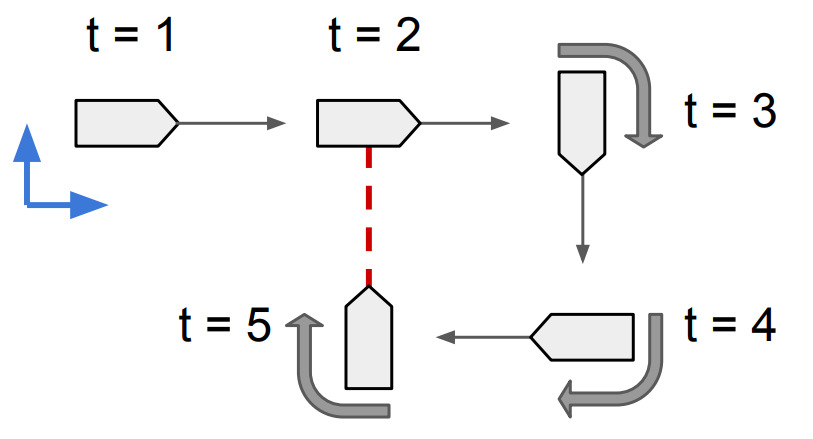
If we want to estimate the vehicle’s poses at times \(t=1,2,3,4,5\), we define the system’s state variables
where \(x_i \in SE(2), i=1,2,3,4,5\) is the vehicle pose at \(t=i\). Then the factor graph models the pose graph problem as
which is shown in figure below.
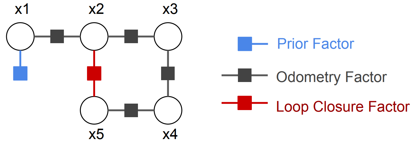
As shown in Eq. (2) and the figure, there are three types of factors: (1) A prior factor, which gives a prior distribution on first pose, and locks the solution to a world coordinate frame. (2) Odometry factors, which encode the relative poses odometry measurements between \(t=i\) and \(t=i+1\). (3) A loop closure factor, which encodes the relative poses measurement between \(t=2\) and \(t=5\).
Python code example
Here we give a Python example on how to use miniSAM to solve the 2D pose graph example.
1. In the first step, we construct the factor graph. In miniSAM data structure FactorGraph is used as the container for factor graphs.
In miniSAM each variable is indexed by a key, which is defined by a character and an unsigned integer (e.g. \(x_1\)).
Each factor has its key list that indicates the connected variables, and its loss function that has covariance \(\Sigma_i\) and optional robust kernel \(\rho_i\) (Cauchy and Huber robust loss functions have been implemented in miniSAM).
In the 2D pose graph example two types of factors are used: unary PriorFactor and binary BetweenFactor.
# factor graph container
graph = FactorGraph()

# Add a prior on the first pose, setting it to the origin
priorLoss = DiagonalLoss.Sigmas(np.array([1.0, 1.0, 0.1])) # prior loss function
graph.add(PriorFactor(key('x', 1), SE2(SO2(0), np.array([0, 0])), priorLoss))

# Add odometry factors
odomLoss = DiagonalLoss.Sigmas(np.array([0.5, 0.5, 0.1])) # odometry measurement loss function
graph.add(BetweenFactor(key('x', 1), key('x', 2), SE2(SO2(0), np.array([5, 0])), odomLoss))
graph.add(BetweenFactor(key('x', 2), key('x', 3), SE2(SO2(-1.57), np.array([5, 0])), odomLoss))
graph.add(BetweenFactor(key('x', 3), key('x', 4), SE2(SO2(-1.57), np.array([5, 0])), odomLoss))
graph.add(BetweenFactor(key('x', 4), key('x', 5), SE2(SO2(-1.57), np.array([5, 0])), odomLoss))

# Add the loop closure constraint
loopLoss = DiagonalLoss.Sigmas(np.array([0.5, 0.5, 0.1])) # loop closure measurement loss function
graph.add(BetweenFactor(key('x', 5), key('x', 2), SE2(SO2(-1.57), np.array([5, 0])), loopLoss))
2. In the second step, we provide the initial variable values as the linearization point. In miniSAM variable values are stored in structure Variables, where each variable is indexed by its key.
# initial varible values for the optimization
# add random noise from ground truth values
initials = Variables()
initials.add(key('x', 1), SE2(SO2(0.2), np.array([0.2, -0.3])))
initials.add(key('x', 2), SE2(SO2(-0.1), np.array([5.1, 0.3])))
initials.add(key('x', 3), SE2(SO2(-1.57 - 0.2), np.array([9.9, -0.1])))
initials.add(key('x', 4), SE2(SO2(-3.14 + 0.1), np.array([10.2, -5.0])))
initials.add(key('x', 5), SE2(SO2(1.57 - 0.1), np.array([5.1, -5.1])))
3. In the third step, we call a non-linear least square solver (like Levenberg-Marquardt) to solve the problem. Result variables are returned in a Variables structure with status code.
# Use LM method optimizes the initial values
opt_param = LevenbergMarquardtOptimizerParams()
opt = LevenbergMarquardtOptimizer(opt_param)

# result variables container
results = Variables()
status = opt.optimize(graph, initials, results)

if status != NonlinearOptimizationStatus.SUCCESS:
    print("optimization error: ", status)
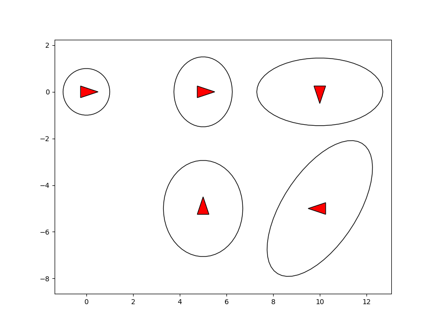
4. In the final step, other than optimized variables we can also calculate marginal covariances of vehicle poses if needed. Calculate marginal covariances we need the graph and optimized variables.
# Calculate marginal covariances for poses
mcov_solver = MarginalCovarianceSolver()

status = mcov_solver.initialize(graph, results)
if status != MarginalCovarianceSolverStatus.SUCCESS:
    print("maginal covariance error", status)

cov1 = mcov_solver.marginalCovariance(key('x', 1))
Finally we plot the estimated vehicle poses with marginal covariance.