2D GPS-like Factor Example
Python and C++ code of this example can be found at gps_factor_example.py and gps_factor_example.cpp respectively.
Here we give a simple example of how to define a 2D GPS-like factor and solve a pose graph problem with GPS-like measurement. The problem is shown in figure below, where a vehicle moves forward on a 2D plane, and has a GPS-like measurement (the translation measurement) at each time stamp,
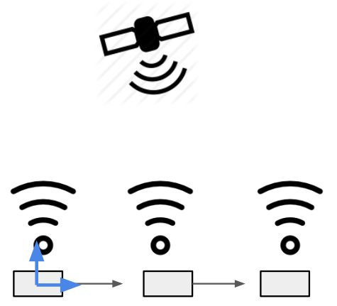
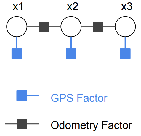
If we define the system’s state variables \(x = \{x_1, x_2, x_3\}\), where \(x_i \in SE(2), i=1,2,3\) is the vehicle pose at \(t=i\). There are three types of factors: (1) Binary odometry factors, which encode the relative poses odometry measurements between \(t=i\) and \(t=i+1\). (2) Unary GPS-like factor, which encodes the translation measurement at every \(t=i\). Then the factor graph models the pose graph problem as
which is shown in figure below.
If we define the GPS-like factor encodes translation measurement which has a Gaussian distribution, the probability distribution of a single factor is defined by
Where \(\Sigma_i\) is the measurement covariance of the Gaussian distribution, and the error function \(f_i(x_i)\) is defined by
Where \(p_x\) and \(p_y\) are X-Y coordinate of vehicle pose \(x_i\)’s translation, and \(m_x\) and \(m_y\) are X-Y coordinate of translation measurement. The Jacobian of the error function is
Python code example
Here we give a Python example on how to define the GPS-like factor.
To define a factor type in Python we need to define a class derived from factor base class minisam.Factor (or minisam.NumericalFactor),
and has following member functions defined:
copy(self): function returns a deep copy of factor.error(self, variables): error function \(f_i(x_i)\), returns error vector as anumpy.array.jacobians(self, variables): Jacobian function \(\frac{\partial f_i(x)}{\partial x}\). return a list of Jacobian matrices innumpy.array. This factor is not needed if this type is derived fromminisam.NumericalFactor, since the Jacobians will be calculated numerically.__repr__(self): function to print the factor, returns a string. This function is optional to define.
We can then define the GPS factor in Python
# GPS translation measurement factor
class GPSPositionFactor(Factor):
    # ctor
    def __init__(self, key, point, loss):
        Factor.__init__(self, 1, [key], loss)
        self.p_ = point

    # make a deep copy
    def copy(self):
        return GPSPositionFactor(self.keys()[0], self.p_, self.lossFunction())

    # error
    def error(self, variables):
        pose = variables.at(self.keys()[0])
        return pose.translation() - self.p_

    # jacobians
    def jacobians(self, variables):
        return [np.array([[1, 0, 0], [0, 1, 0]])]

    # optional print function
    def __repr__(self):
        return 'GPS Factor on SE(2):\nprior = ' + self.p_.__repr__() + ' on ' + keyString(self.keys()[0]) + '\n'
The factor graph of this example can be built by
# factor graph container
graph = FactorGraph()

# Add odometry factors
odomLoss = ScaleLoss.Scale(1.0) # odometry measurement loss function
graph.add(BetweenFactor(key('x', 1), key('x', 2), SE2(SO2(0), np.array([5, 0])), odomLoss))
graph.add(BetweenFactor(key('x', 2), key('x', 3), SE2(SO2(0),np.array([5, 0])), odomLoss))

# Add the GPS factors
gpsLoss = DiagonalLoss.Sigmas(np.array([2.0, 2.0])); # 2D 'GPS' measurement loss function, 2-dim
graph.add(GPSPositionFactor(key('x', 1), np.array([0, 0]), gpsLoss))
graph.add(GPSPositionFactor(key('x', 2), np.array([5, 0]), gpsLoss))
graph.add(GPSPositionFactor(key('x', 3), np.array([10, 0]), gpsLoss))
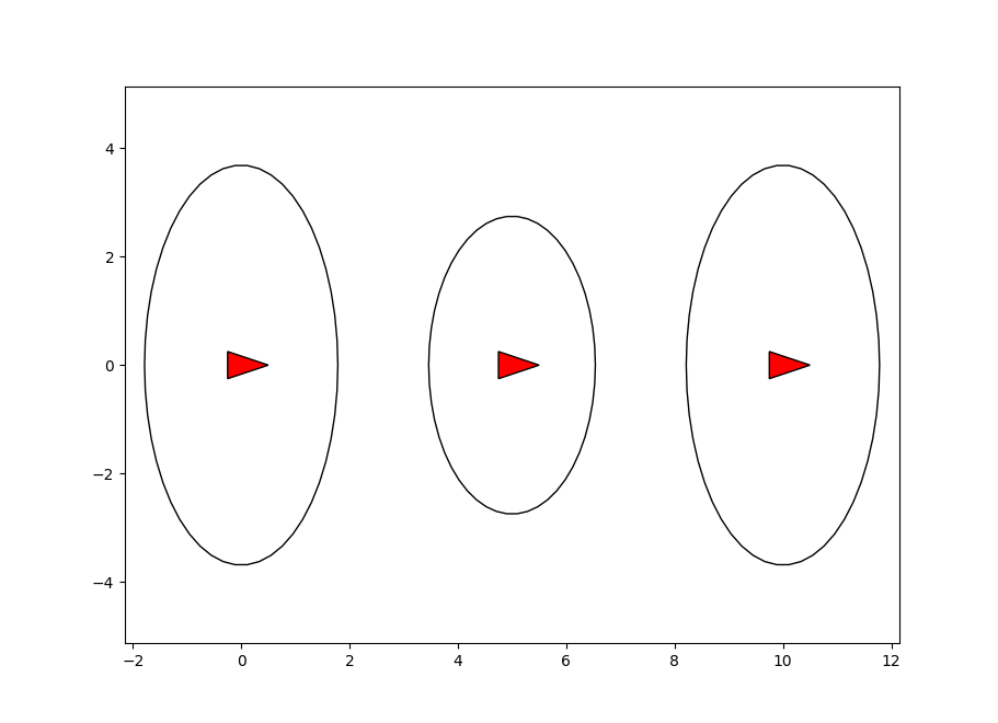
Finally we can optimize the factor graph, and plot the estimated vehicle poses with marginal covariance.